Statistics Unit 6: Mean Comparisons: T-Test, ANOVA
Section 1: Tests of Contrast
Unlike correlations, which tell us the relationship between two variables, we often want to know if there are meaningful difference between two groups. These can be existing groups (for examples: IQs of people born in December and June; blood pressure) or groups we’ve experimentally created (for example: two classes taught material using different methodologies; people treated with two different kinds of medication for a specific illness).
Tests of contrast begin with the null hypothesis that there is no difference between the true population means of the groups. We then take samples from each group and use the means and distributions of those samples to calculate the probability that we could see the differences we got in our experiment if the groups were actually the same.
As with all statistical testing, if that p-value is less than α, we reject the null hypothesis and say the groups are different. If the p-value is greater than α, we fail to reject the null hypothesis.
Because individual students’ understanding of these topics tends to vary, I have included some videos that cover the very basics of the topic to help anyone struggling with getting the concepts down. If you have a more advanced understanding, feel free to skip these videos as noted in the text.
Section 2: t-test
The t-test is one common test of contrast for two groups. We start with the null hypothesis that there is no difference between groups (i.e., the groups are the same). If the groups are the same, then when we take a number samples from each group, we should see roughly the same mean. But we expect because we are sampling a smaller population, that we might see some difference even if the groups are really the same.
Let’s say for example, I want to see if there is a difference in test scores between people sitting on the right side of the room and people sitting on the left. Barring some other factor like the smart students sitting together or some other non-randomness in seating (a potential confounding variable), you would expect that these groups are identical. They are in the same class, they are made up of the same type of population, etc. However, if I randomly chose 5 students from the right and 5 students from the left and found the mean scores of each group, it’s not all that likely that the mean scores would be identical. The question then is, how different do they need to be to consider it meaningful.
The t-test is a little more complex mathematically, but it effectively just looks at the difference in mean scores of the two experimental groups relative to the standard deviation. If the difference in means is large and the standard deviation is small, this would seem like a true difference between the groups. If the difference in means is small and the standard deviation is large, we are not very confident that this is a true difference.
Below is an example of an experiment with two groups, group A and group B. Individual points correspond to the individual data in the groups. The X axis corresponds to the data values. The y-axis is just for the illustration of the data distribution curves.
Source: https://serc.carleton.edu/introgeo/teachingwdata/Ttest.html
You might notice that many of the red and blue points overlap in values. Overall, the mean of the blue is lower than the mean of the red, but many individuals in the blue group had a higher score than many individuals in the red group. The mathematical question is then if it’s the case that the true populations of the blue and red were actually identical, what are the odds that we could have gotten these results. If those odds (the p-value) are less than α, we say these groups are significantly different. If p>α, we say that we found no statistical difference between the two.
Let’s take a look at mean and variability:
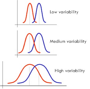
Source: http://esa21.kennesaw.edu/modules/basics/exercise3/3-8.htm
In each of the cases, the mean of the red and the mean of the blue are constant. If the distributions look like the above, you can imagine that if we draw randomly from these groups, the difference between groups will be clearer in the low-variability (low standard deviation) case than the high-variability (high standard deviation) case. We will have fewer overlapping points in our sample populations.
This is a little long, but it’s an exceptionally clear explanation of the process of doing a t-Test. (He does talk about “accepting” the null hypothesis, which is not precisely correct, but is, as we have covered, pragmatically correct.)
This is not required for the course, but if you want a little more in-depth look at the mathematics and implementation of the test in software, this video is a good resource.
Section 3: Types of t-tests
There are several types of comparisons possible in t-tests:
Independent Samples: There is no logical way to pair samples between the two groups. If we conducted our earlier IQ tests based on birth month, we have a group of December-born participants and a group of June-born participants. The individuals in each group were randomly selected and no individual in one group has any special relation to any individual in the other group.
It is not necessary to watch the demo, but if you would like a detailed example, this is a good one:
Dependent Samples Matched: There is a special logical tie between individuals in each group. If instead of birth month, we wanted to compare the IQs of first-born children with second-born children, choosing pairs from families so that for each first-born child in the first group, there is a corresponding younger sibling in the second group. If we are interested in the differences between the two groups, we can just mathematically look at the relationships between the paired participants, thereby eliminating other effects like socioeconomic status or education. This makes it easier for us to identify effects correctly. It reduces the chances of making an error due to confounding factors.
Dependent Samples Repeated Measures: Instead of pairing of different individuals in the two groups, the two groups are comprised of the same subject measured in two different conditions. This may be before and after education, a change in diet, or just practice performing a task.
It is not necessary to watch the demo, but if you would like a detailed example, this is a good one:
One Sample: The one sample t-test is used to determine whether a sample could have been generated by a process with a specific, known mean. For example, if you have a machine that is filling orange juice cartons with 32 oz. of orange juice, you could test the output of that machine to make sure it is within operating expectations.
It is not necessary to watch the demo, but if you would like a detailed example, this is a good one:
Section 4: Analysis of Variance (ANOVA)
The t-Test can only be performed for two groups. When we want to look for differences in three or more groups, we instead use other tests of contrast, most commonly, the analysis of variance (ANOVA). As noted earlier, the variance is just the standard deviation squared. Conceptually, you can consider variance and standard deviation to examine the same type of measure — roughly the average distance of an individual from the mean.
ANOVAs are useful for when you want to see if there are differences among the means of groups.
If the setup for ANOVAs is not clear, this is a lengthy, but very clear video about when we might use an ANOVA. It is very basic, so feel free to skip it if you understand conceptually how the t-Test two-group comparison is simply being expanded to three or more groups. (No mathematics in the video.)
ANOVAs work by taking a look at the variance of the individual groups and comparing it with the variance of the aggregate of all groups. That is, we take all of the individual data from each of our groups and place into one large aggregate. If the null hypothesis that there is no difference among the groups is actually true, then the aggregate group mean and variance will be the same as the individual groups. If the groups differ, the aggregate distribution will encompass them all and will have a larger variance than the individual groups.
Likely significant differences case – Generated from code at: http://www.statistics4u.com/fundstat_eng/dd_distributions_combi.html
The image above shows several distributions of data from different groups (in different colors) and the aggregation of all of the data from all groups (in black – note: raised higher on the y-axis just for illustration and separation of the groups). The important thing to note when performing an ANOVA is the variance (or again, if it is easier, just think about the standard deviation) of these distributions. The ANOVA tests whether the variance of the aggregate group (in black) is larger than the variance of the individual groups. In this case, it appears that the aggregate distribution is a lot wider than the width of any of the individual groups. That would indicate that there is likely some real difference among the groups.
If instead, the individual groups were exactly identical to one another, the above plot would instead look like:
no significant differences case – Generated from code at: http://www.statistics4u.com/fundstat_eng/dd_distributions_combi.html
In this case, all of the distributions are on top of one another (so you can’t see them) and the variance of the aggregate (in black) is identical to the variance of the individual distributions (in colors, but not visible as they are all overlapping).
The statistic used for ANOVAs is called the F-test statistic.
Basically: F = variance of aggregate of data / variance of individual groups
In the first case, F would be large. In the second case, F would be small. Large values of F result in small p-values (dependent also on sample size) and small values of F result in large p-values.
Section 5: Post-hoc/paired comparisons
An ANOVA provides insight into the null hypothesis that there is no difference among the multiple groups. For a t-Test, if we reject the null hypothesis, we know that the two groups differ, but with an ANOVA, does rejecting the null hypothesis mean that all three (or more) groups differ from one another, or just that one group differs from the other two?
The test itself does not provide this information. If we reject the null hypothesis that there is no difference among groups, we simply know that there is some difference among the groups. We can do post-hoc testing to gather further details. Post-hoc tests (often also called paired comparisons) are performed by breaking down the groups into all possible pairings and running tests (often t-Tests or similar) on each pair. After the paired comparisons are performed, we then know which groups differ significantly from one another.
So, for example, if we had three classes, each taking a statistics exam and the means of the classes were class1=75, class2=76, and class3=55, we might perform an ANOVA and find a low p-value, indicating that there is likely some real difference among the classes. However, we would not know more details than that.
Post-hoc comparisons would be:
class1 vs class2
class1 vs class3
class2 vs class3
These comparisons, like all of our other statistical testing would result in a p-value, which we would compare with our selected α.
We might see in our individual comparisons that there is a significant difference between class1 and class3, and a significant difference between class2 and class3, but no significant difference between class1 and class2. We can only run these additional comparisons IF the initial ANOVA showed a significant difference.
One important element of post-hoc testing is maintaining α appropriately. If you were to conduct multiple tests, each with a 5% chance of making a type-I error, you would increase the chances of making an error among all of the tests. Post-hoc testing uses correction factors to ensure that the total chance of error remains 5%. There are many different approaches to this depending on a variety of factors including independence of tests. The details of this are built in to statistical software. We will not cover it more extensively than just the concept above.
Section 5: One-tailed and two-tailed testing
Note: this section applies to many types of statistical testing. It is especially an important parameter of ANOVAs, t-Tests.
When we conduct experiments, sometimes we are only interested in one outcome direction. For example, if we want to see if a new educational method is better than an existing one, we really just want the null hypothesis to be that the new method is not better than the old method. Not only is the new method not useful if it’s just the same effectiveness as the old method, but it’s certainly not useful if it’s worse. Thus, we can elect to choose to look for only an outcome in which the new method is better and accept that our test will not identify outcomes in which the new method is worse.
This is important because when we usually conduct tests, especially tests of contrast, we only determine whether there is a difference between the two groups. Thus, if we allow for a 5% chance of making a type-I error (α=0.05), we are really actually allowing for a 2.5% chance in each direction (a 2.5% chance our new method was better and a 2.5% chance our new method was worse).
That is, we are allowing a 2.5% chance that the new method randomly looks better than the old method and a 2.5% chance that it randomly looks worse even when they are actually the same. Because we are considering either direction, this is called a two-tailed test. We are looking for results in either tail of the distribution.
If instead, if we are only interested in one direction, we can maintain our 5% chance of making a type-I error, but reduce our chance of making a type-II error by only looking at one tail. That is, we move the whole search area over to one side. Such a test will not give us any information about effects in the other direction.
We will again not cover this extensively, but when selecting analysis criteria in software, it is important to decide if the test is two-tailed or one-tailed. That is, do we care about outcomes in either direction or only in one.
Let’s say, for example, we want to compare your scores in statistics class this year with the previous year’s scores to see if the new additions to the notes and approaches improved the class.
Two-tailed null hypothesis: there is no difference in score between last year’s class and this year’s class.
A significant outcome of this test could then be that this year’s class performed significantly better OR that this year’s class performed significantly worse.
One-tailed null hypothesis: this year’s class did not perform better than last year’s class
A significant outcome of this test could only be that this year’s class performed significantly better than last year’s class.