Statistics Unit 5: Inferential statistical testing and Correlation
We’ve learned all about collecting sampled information in an experiment and using descriptive statistics to look at the mean and standard deviation of the results. We are now ready to start examining about how inferential statistics works!
Section 1: Basics of Inferential Statistical Testing
Everything in inferential statistics is based on a very simple question:
P-value
Statistical tests work by mathematically computing the answer to that question. That is, we use mathematical methods to find the probability that the results obtained in the experiment could have happened by chance if the null hypothesis were actually true (which is something we can never be sure about). We call this probability the p-value. We typically write it in decimal form rather than percentage form, so while the probability of something will range from 0% to 100%, when we report p-values, we typically list them as ranging from 0.000 to 1.000. If the probability that our results could have happened by chance was 5%, we would say p=0.05.
A low p-value means the results were unlikely to have happened by random chance, and so we should maybe consider them to be “real” effects or findings.
α (alpha)
While calculating the probability that our results could have happened by chance is a useful start, we need to set up a criterion for deciding how to consider the results of that calculation. In the scientific method, we set our criterion, called α, to be some percentage chance of error that we feel comfortable accepting, and use that as our determination of whether a result is sufficient to reject the null hypothesis or not. If we feel comfortable accepting that a 5% chance of randomness is low enough, we would say α=0.05.
How does “Significance” work?
Let’s say we want to do an experiment to compare IQs for people born in December and June. We would first set up the null hypothesis and the criterion:
Null hypothesis: There is no difference in IQ scores for people born in December and June.
Almost undoubtedly, if we conduct IQ tests on 20 people born in December and 20 people born in June, the average scores will be at least slightly different, even if by chance. We’re very unlikely to get exactly the same scores. So, even if the null hypothesis is actually true. While I have not conducted the study and while we would need to test everyone in the world to be certain, I would expect that it actually is true. And remember, until we have sufficient evidence to reject the hypothesis, we are obligated to assume it is true.
We then select our test criteria arbitrarily. We might choose α=0.05, which means that in our experiment, when we see a difference between the two groups that was 5% or less likely to have occurred by chance if the null hypothesis were true, we will then reject the null hypothesis and say that there is a significant difference between the two groups.
The term “significant” means exactly this, that our p-value (the probability that the results we got could have happened by chance if the null hypothesis were true) is less than our criterion α. If this feels uncomfortable, there is good reason. We are going to be wrong sometimes!
Section 2: Correct Decisions and Mistakes
By definition, we might consider a result “real” by mistake or we might miss a “real” result. There is a tradeoff based on how strict we are with our criteria. We have a formal way of defining mistakes in statistical methodology.
Type-I/type-II errors
There are no specific rules about what α must or even should be. In standard scientific practice, it is common to choose α=0.05 or α=0.01; that is, we are willing to reject the null hypothesis and say there is a significant difference between the two groups, even when there is a 5% (or in the case of α=0.01, a 1%) chance that the results just happened by chance and no difference actually exists. That means, for α=0.05, we’re willing to be wrong 1 out of 20 times. So, why not be more cautious, and make α=0.0000000001 or something very tiny? Well, sometimes we do this in experiments, but we then face the opposite problem. We will fail to reject the null hypothesis when it is actually false.
In testing, these are known as type-I and type-II errors.
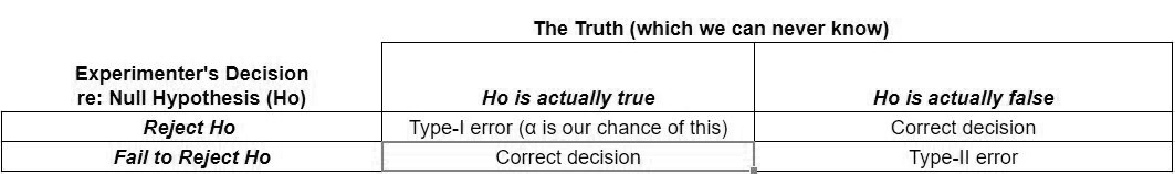
A type-I error is when we choose to reject the null hypothesis, but in fact the null hypothesis was true. So, for a particular experiment, by selecting our α criterion, we choose the probability of this happening. If we choose α=0.05, we are accepting that when we conduct our experiment, we have a 5% chance of making a type-I error. In our IQ example, this would mean that we’ve chosen to reject the null hypothesis that there is no difference in IQ based on birth month. We would say there is a significant difference based on birth month. It is understood in scientific language that “significant difference” means that we got a result that is below some threshold of error. In this case, the result we got showed less than a 5% chance of occurring randomly if the null hypothesis were true. So, that is sufficient to reject the null hypothesis and claim it is false. We know that when we report this significant difference, claiming that IQs for people with December and June birthdays differ includes a 5% chance that we are wrong.
It is important to understand that we can never know that we are actually wrong , we just know that there is a 5% chance that we could be wrong by rejecting the null hypothesis (made a type-I error).
But what if there really is a difference in IQs between people born in December and June? If we reject the null hypothesis, then we are correct and have not made an error. If instead, we run our experiment and get a p-value greater than α, we then would “fail to reject” the null hypothesis. If there really is a difference in the true population means and we fail to reject, we are then making a type-II error. That is, there is really a difference, but we have failed to find it. While α tells us the likelihood we will make a type-I error, knowing how likely it is that we might make a type-II error (known as β) is much more difficult. There are methodologies for estimating β, but they are far less rigorous and certain than α, which is definitively known because we have defined it in our experiment.
However, there is one thing we can say for certain, α and β are interrelated. If we raise α, we increase our risk of making a type-I error, but decrease our risk of making a type-II error. If we lower α, we decrease our risk of making a type-I error, but increase our risk of making a type-II error. And while we specifically set the chances of making a type-I error when we choose α, and thus it is fixed, collecting more data reduces the chances of making a type-II error. So, overall, a larger sample size minimizes our chances of making an error.
During our upcoming experiment, the probability of making a type-I error will be α. There is some probably of making a type-II error, β, but it’s not easy to exactly quantify. The only thing we know about β is that as α decreases, β increases and as α increases, β decreases. If we make our criteria less strict (raising α), we’re less likely to miss an effect.
If p<α, we will reject the null hypothesis and the probability that we’ve made a type-I error is equal to p, which represents the probability the results we’ve seen in the experiment could have happened by random chance.
Because we’ve rejected the null hypothesis in this case, we know we did not make a type-II error.
If p>α, we will fail to reject the null hypothesis and therefore, because we have failed to reject the null hypothesis, we know we did not make a type-I error.
Because we’ve failed to reject the null hypothesis in this case, we might have made a type-II error, however, it is difficult to quantify exactly.
Section 3: Trial by jury
The United States trial-by-jury process works very much like the scientific method. The null hypothesis is that the defendant has not committed a crime. The prosecutor then tries to provide sufficient evidence that the defendant did indeed commit the crime. If evidence is sufficient and meets the jury’s criteria, the null hypothesis will be rejected and the defendant is found guilty.
The language and logic are structured the same way as scientific method (and all other proper logical inquiry). We begin with the null hypothesis, provide evidence, the jury evaluates that evidence to determine the likelihood of that evidence assuming the null hypothesis is true (the defendant is innocent). If the likelihood (although this is not done mathematically, it is equivalent to a p-value) is sufficiently low to fall below “reasonable doubt” (equivalent to α), then the null hypothesis is rejected and the defendant is guilty. If the evidence is not sufficient to reject the null hypothesis and find the defendant guilty, they are notably NOT declared to be innocent. Instead, they are found “not guilty.”

This may seem like a subtle point, but it speaks to the function of the null hypothesis and burden of proof (as discussed in a previous unit). A “not guilty” finding is actually not a declaration of innocence, as that was not directly assessed, but rather a statement that the prosecutor, who had the burden of proof, failed to meet the criteria with evidence, and therefore, we continue the obligation of assuming the null hypothesis is true.
In trial terms, if the jury wrongfully convicts a defendant, that is a type-I error. If the jury fails to convict a defendant who did actually commit the crime, that is a type-II error. Both our criminal justice system and the scientific method are designed to somewhat favor type-II errors over type-I errors. That is to say, we would tend to “rather” fail to make a conclusion than draw a false conclusion.
Section 4: Reporting results
This system can result in confusing interpretations of results. In our IQ study, we would either say, “there is a significant difference between the IQs of people born in December and people born in June,” or “there is no significant difference between the IQs of people born in December and people born in June.” Despite sounding symmetrical, those do not really have symmetrical meaning.
“There is a significant difference…” means that the results we got in our study had a probability of less than α of occurring if the null hypothesis were true (there is no difference between the groups). This tells us something about how likely it is that the null hypothesis is false.
“There is no significant difference…” simply means that in our study, the differences we saw had a greater than α chance of occurring randomly if the null hypothesis were true. You might be surprised when I say that this tells us almost nothing about how likely it is that the null hypothesis is true.
For one thing, the size of our study matters. If we see a small difference between the two groups, but we’ve only tested a small number of people, the probability that we got that small difference by chance will be high. If we have tested a large number of people, that small difference becomes more reliable and the probability that it occurred by chance decreases.
Remember when we talked about standard error of the mean, an estimate of how close our experimental mean is to the true population mean. If the null hypothesis is actually false, the p-value for just about any study conducted will be higher for a smaller study than a larger study. As we gather more information, we know more. So, therefore, a higher p-value DOES NOT tell us that it is more likely that the null hypothesis is true, but rather more just tells us that we don’t have enough information.
There is a complex consideration in the way all of this works. What happens if you conduct a study and find that p=0.051, which is larger than α=0.05?As you know, this means you fail to reject the null hypothesis. However, it also means that the results you got in your experiment only had a 5.01% chance of happening randomly, and most likely, the null hypothesis is actually false. In fact, even if you got p=0.49, there was still only a 49% chance of having gotten those results if the null hypothesis were true. So, more likely than not, the null hypothesis is not true!
“Facts are stubborn, but statistics are more pliable.” – Mark Twain
Thus, we have to be extremely careful about drawing conclusions from failing to reject the null hypothesis because we have set up arbitrary and strict criteria that result in favoring type-II errors over type-I errors.
Let us say in our IQ study, we found that p=0.03; that is, there is a 3% chance that the difference between December-born and June-born IQs that we saw in our study occurred randomly. If we chose to set α=0.05, p is less than α and we would reject the null hypothesis and state that there is a significant difference. If we chose to set α=0.01, p is greater than α and we would fail to reject the null hypothesis and say there is no significant difference. This is why the structure of the scientific method is strictly that we assume the null hypothesis to be true until burden of proof is met, and we cannot directly conduct studies that prove the null hypothesis.
Why can’t we conclude much from failure to reject?
Imagine, going back to unit 1, if we conducted a bigfoot expedition. The expedition team doesn’t really want to search very hard, so they just look in one spot and call it a day. (This is equivalent to a small sample size.) Would you be convinced that because they didn’t find evidence of bigfoot (the experiment has a high p-value), it would be okay for them to write a scientific paper claiming that bigfoot doesn’t exist based on their search?
While we may not have real evidence that bigfoot exists, what if I conducted a far more mundane study to determine whether anyone lived on my street. In my experiment, I look out the window one time (small sample size) and don’t see anyone (high p-value). Have I demonstrated that no one lives on my street? What if I look outside every hour for a week (bigger sample size) and still see no one? That is getting more convincing. How many times do I need to look before we are certain that no one lives on my street? As again, this is not an easy question to answer, we assume the null hypothesis until evidence is found. If I see no one, that would be a very high p-value. What if I see someone drive by? What if I see someone walk by, but not enter their house? What if I see a light on in a house? What if I see someone enter a house? What if I meet someone who tells me they live in the house across the street? As we gather more and more evidence, our p-value goes down and we will, based on some criteria, reject the null hypothesis that no one lives on the street. If we continue searching and still find no evidence, our p-value remains high, but we feel better about our failure to reject the null hypothesis.
If we are conducting multiple tests, it is important to understand that overall, we are then increasing the risk that we are going to make a type-I error. If we conduct one test with α=0.05, then the chances of making a type-I error are 5%. If we conduct two independent tests, the chances of making at least one type-I error are 9.75%, and if we conduct twenty tests, the chances of making at least one type-I error are 64%. Note that this is a result of probabilistic math. You may be tempted to simply add the percentages and say that if the chances of making an error on one test is 5%, then the chances on two tests should be 10%. However, if you imagine this line of thinking with 21 tests, the chances would then be 105%, which doesn’t make sense. Instead, you must calculate 100% – the chances of making no errors.
Section 5: Correlation
“Math is a language that you use to describe statistics, but really it’s about collecting information and putting it in an order that makes sense.” – Lauren Stamile
Statistical testing can take on many different specific forms, but a very large portion of the types of test we might like to look at fall into a small number of categories. The next few units will all cover different types of test.
Correlation
Correlation is a test of the relationship between two (or more) variables that extends across a range of inputs and outputs. We typically manipulate an independent variable across a range of levels and determine whether it has an impact on a dependent variable.
For example, we could conduct an experiment to see if the amount of water we give a certain type of plant has an impact on its height.
Other related factors can be negatively correlated. That is, as one increases, the other decreases. If we look at miles traveled vs. amount of gasoline in a car’s tank, we would see that as more miles are traveled, amount of gas in the tank decreases.
Correlation testing will mathematically result in a p-value indicating the probability of seeing the results we have seen if no real relationship exists (if the null hypothesis were true). So, if we were to conduct our study to determine whether the amount of watering affects plant height, the null hypothesis would be that amount of water does not have any relationship with plant height.
The mathematical process for calculating correlation results in a correlation coefficient, R, which essentially describes how many data points gathered in the experiment fall onto a perfect straight line. If all of the data points fall exactly on a line and there is a positive relationship (as one grows the other grows), R will be equal to 1. If all of the data points fall exactly on a line and there is a negative relationship (as one grows the other grows), R will be equal to -1. The positive or negative part of the number just indicates the direction of the relationship. The value of R indicates how orderly the data are relative to a straight line. If changes in the independent variable are not associated in a meaningful way with the dependent variable at all, R=0.
Below is a set of scatter plots (x-axis is the independent variable [amount of water, for example], y-axis is the dependent variable [plant height, for example], and each point represents one plant) showing a range of values for R. The higher the value is for R, the more certain we are that the relationship between the two variables is meaningful.
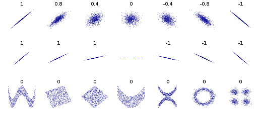
R values for different scatters. From https://en.wikipedia.org/wiki/Correlation_and_dependence
Notice that the orderliness and not the slope of the line is the key element. The top row shows sets of data with the same slope, but different “orderliness” and different R values. The middle row shows sets of data with different slopes, but the same “orderliness” and the same R values. The only exception is the flat line, which also may look orderly, but indicates no meaningful relationship between variables. The bottom row shows other examples of unrelated variables.
Datasets with the same R-value and p-value can look very different. Below is a set of graphs showing four sets of data with the same correlation of 0.816
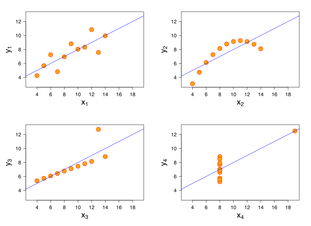
Four sets of data with the same correlation of 0.816. From: https://en.wikipedia.org/wiki/Correlation_and_dependence#/media/File:Anscombe%27s_quartet_3.svg
The following table shows the value of R necessary to be considered significant for α values of 0.05 and 0.01 (shown as the R value for which p=α – for example, when R=0.707 and N=8, p=0.05; any R>0.707 will result in a p<0.05).
The first column is the degrees of freedom, which is closely related to the sample size, but is a measure of the part of the sample that is mathematically useful. In the case of a correlation, if we collect only two samples, it is not meaningful. That is because we can always connect those two points with a line that they both will fall on perfectly. It is only when we add a third point, that we start getting meaningful information about the relationship between the variables. Therefore, in the case of correlations, the degrees of freedom (or the meaningful information) is the number of samples collected minus 2. We won’t cover this concept extensively.
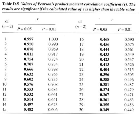
So, as another example, according to this chart, if α=0.05 (that is, we are okay with a 5% chance of making a type-I error in our study), for a sample size (N) of 3, R must be greater than or equal to 0.997 in order for us to reject the null hypothesis. For the same α and a sample size of 32, R must be greater than or equal to 0.349 in order for us to reject the null hypothesis. While these are positive numbers, negative magnitudes would be the same. The negative sign only indicates the type of relationship. So, the null hypothesis would be rejected for R less than or equal to -0.997 and -0.349 respectively in the previous examples.
Section 6: Magnitude
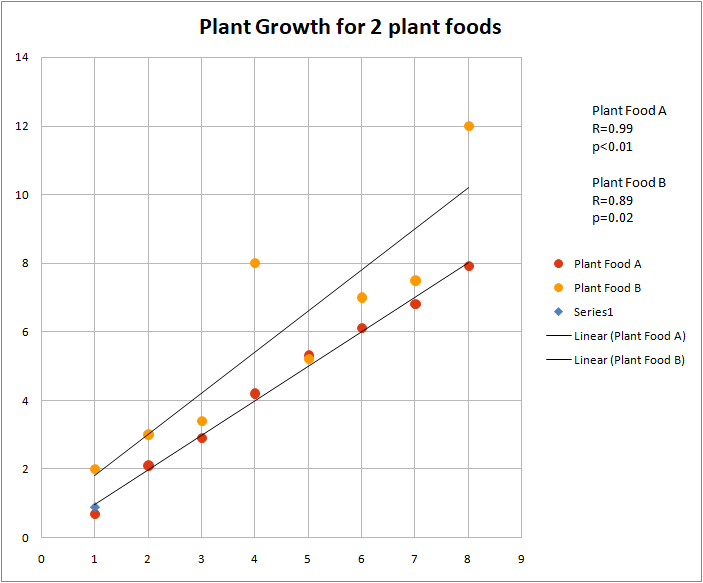
Below is an example of a graph showing plant growth from 2 different plant foods. Note several things:
- For every amount of plant food, feeding the same amounts of plant food A and B to plants always resulted in bigger plants when fed B.
- Plant food B growth is less consistent in terms of effect, so R is lower and p is higher.
- If you had chosen α=0.01, the effect of plant food B would not have been found to be signficant.
- Given the choice, I would always feed my plants B.
Section 7: Causation
One famous (and famously misused science-denial) saying is that “correlation does not imply causation.” That is to say, we may search and find mathematical relationships between variables that do not have real meaning. In most experiments, this is carefully considered and noted. However, it is possible to find these mathematical relationships that do not have meaning, covered in a previous unit, again called spurious correlations.
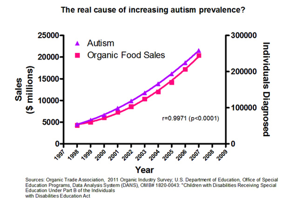
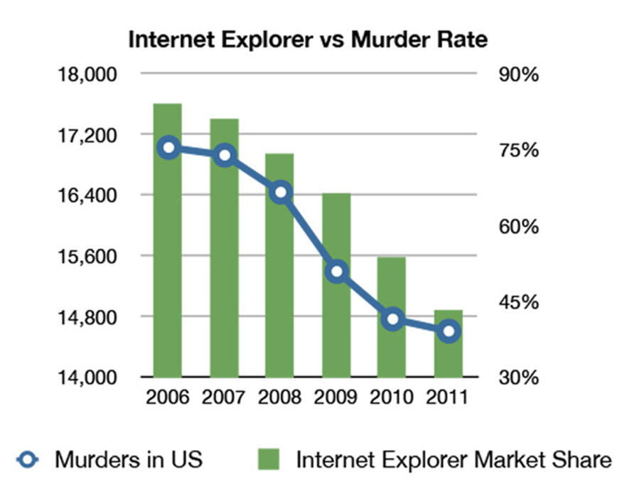
There are many famous joke examples of spurious correlations on the Internet (again, we looked at some in the previous unit, but now you have additional context, so you may wish to look back), ranging from estimated relationships between the number of pirates sailing the high seas and global temperature (along with the tongue-in-cheek claim that the lack of pirates is causing global warming) to detailed measurements showing a relationship between the rise in organic food sales and autism diagnoses, Nicolas Cage films released each year and swimming pool accidents (R=0.67), and letters in the winning words of the National Spelling Bee and deaths caused by venomous spiders (R=0.81). It also turns out that Internet Explorer market share and murder rate in the US are negatively correlated, Mexican lemon imports and highway deaths are negatively correlated, and perhaps most surprisingly, average serum cholesterol fell when Justin Bieber was born, but grew once more after Facebook was released (the satirical headline: Facebook cancels out the cholesterol-lowering effects of Justin Bieber).
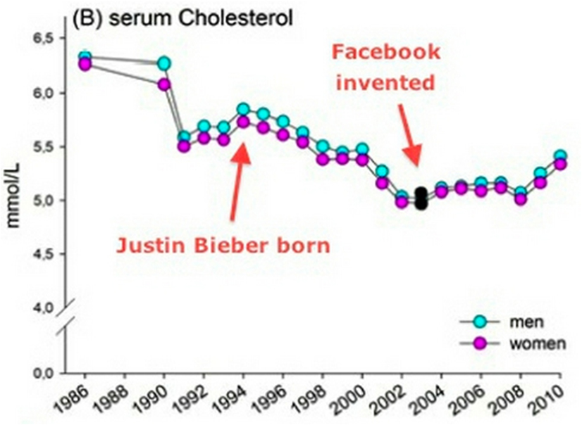
Facebook cancels out the cholesterol-lowering effects of Justin Bieber – source: unknown
Source unknown
We might be hard pressed to get a paper published claiming that Nicolas Cage films were responsible for swimming pool accidents, but that does not stop people from identifying somewhat less ridiculous sounding trends and attempting, without evidence, to claim they are related. As a result, correlations are carefully evaluated and attempts to remove or consider other factors are made in studies in order to prevent spurious results.
The above examples are completely unrelated factors that happen to mathematically correlate, but there are also times when two variables are actually related to a third variable, rather than each other. This is known as a third-factor (or common-cause) relationship. For example, we might observe that during the Summer months, there is a rise in ice cream consumption and a rise in the frequency of mosquito bites. It might be tempting to say then that eating ice cream attracts mosquitos, but in fact, both ice-cream consumption and mosquito presence are associated with a third factor, the seasonal climate.
Section 8: Calculating Correlations
We are focused here on the underlying theory and interpretation of statistical testing, but if you wish to know how to do correlation calculations, here are a few tutorials that will help.